#
Dr. M. Baron, Statistical Machine Learning class, STAT-427/627
# DEEP LEARNING
1.
Artificial neural network with no
hidden layers is just linear regression
Artificial neural networks are available in package neuralnet.
> library(neuralnet)
Create the training and testing data.
> attach(Auto)
> n = length(mpg)
> Z = sample(n,200)
> Auto.train =
Auto[Z,]
> Auto.test =
Auto[-Z,]
> nn0 = neuralnet( mpg ~ weight+acceleration+horsepower+cylinders, data=Auto.train, hidden=0 )
> nn0
Error Reached Threshold Steps
1 1720.963134
0.009532195866 8565
> plot(nn0)
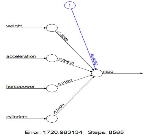
This is the linear regression! Weights are slopes, and the intercept
is shown in blue.
> lm( mpg ~ weight+acceleration+horsepower+cylinders, data=Auto.train )
Coefficients:
(Intercept) weight
acceleration horsepower cylinders
44.446611467
-0.005475864 0.056149012 -0.015172364
-0.744442628
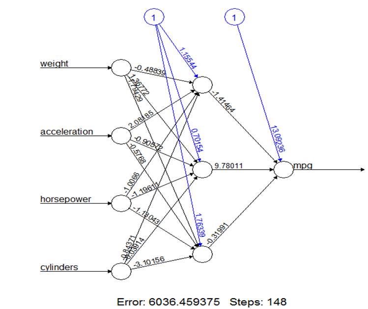
2.
Artificial neural network
Now, introduce 3 hidden nodes.
> nn3 = neuralnet(
mpg ~ weight+acceleration+horsepower+cylinders, data=Auto.train, hidden=3 )
> plot(nn3)
3.
Prediction power
Which ANN gives a more accurate prediction? Use the test data for comparison.
> Predict0 = compute( nn0, subset(Auto.test,
select=c(weight, acceleration, horsepower, cylinders) ) )
This prediction consists of X-variables “neurons” and predicted
Y-variable “net.result”.
> names(Predict0)
[1] "neurons" "net.result"
> mean( (Auto.test$mpg
- Predict0$net.result)^2 )
[1] 18.83350028
Prediction MSE of this ANN is 18.83.
> Predict3 = compute( nn3, subset(Auto.test, select=c(weight,acceleration,horsepower,cylinders)
) )
> mean( (Auto.test$mpg
- Predict3$net.result)^2 )
[1] 61.84868054
Its 3-node competitor has a much higher prediction MSE.
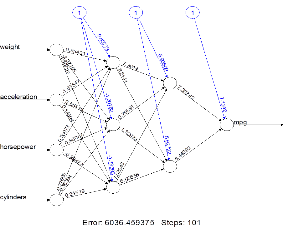
4.
Multilayer structure
The number of hidden nodes can be given as a
vector. Its components show the number of hidden nodes at each hidden layer.
> nn3.2 = neuralnet(
mpg ~ weight+acceleration+horsepower+cylinders, data=Auto.train, hidden=c(3,2) )
> plot(nn3.2)
5.
Artificial neural network for
classification
> library(nnet)
Prepare our categorical variables ECO and ECO4
> ECO = ifelse( mpg > 22.75, "Economy",
"Consuming" )
> ECO4 = rep("Economy",n)
> ECO4[mpg < 29] = "Good"
> ECO4[mpg < 22.75] = "OK"
> ECO4[mpg < 17] = "Consuming"
> Auto.train = Auto[Z,]
> Auto.test = Auto[-Z,]
Train an artificial neural network to classify cars into “Economy”
and “Consuming”.
> nn.class = nnet(
as.factor(ECO) ~ weight +
acceleration + horsepower + cylinders, data=Auto.train,
size=3 )
#
weights: 19
initial value 169.471585
final value 138.379332
converged
> summary(nn.class)
a 4-3-1 network with 19 weights
options
were - entropy fitting
b->h1 i1->h1 i2->h1 i3->h1
i4->h1
-0.11
-0.35 0.12 0.32
0.16
b->h2 i1->h2 i2->h2 i3->h2
i4->h2
0.59
-0.37 -0.56 0.67
0.44
b->h3 i1->h3 i2->h3 i3->h3
i4->h3
0.50
0.16 0.41 -0.49
0.02
b->o h1->o h2->o h3->o
-0.12
-0.27 0.03 0.02
This ANN has p=4 inputs, one layer of M=3 hidden nodes, and a single (K=1)
output. We need to estimate M(p+1)+K(M+1) = (3)(5)+(1)(4) = 19 weights.
Classification into K > 2 categories is similar.
> nn.class = nnet(
as.factor(ECO4) ~ weight+acceleration+horsepower+cylinders,
data=Auto.train, size=3 )
# weights:
31
initial
value 333.799856
final
value 276.956630
converged
> summary(nn.class)
a 4-3-4 network with 31 weights
options were - softmax
modelling
b->h1
i1->h1 i2->h1 i3->h1 i4->h1
0.39 0.69 -0.58
0.23 0.11
b->h2
i1->h2 i2->h2 i3->h2 i4->h2
-0.49
-0.67 -0.65 -0.68
0.11
b->h3
i1->h3 i2->h3 i3->h3 i4->h3
-0.67
0.24 0.59 0.43
0.00
b->o1
h1->o1 h2->o1 h3->o1
0.98 -0.25 0.32
-0.12
b->o2
h1->o2 h2->o2 h3->o2
0.13 0.41 0.19
-0.02
b->o3
h1->o3 h2->o3 h3->o3
0.20 0.28 0.34
-0.01
b->o4
h1->o4 h2->o4 h3->o4
-0.24
0.42 -0.09 0.41
Here K = 4 categories, so we are estimating (3)(5) + (4)(4) = 31
weights.